Exploring the Oddities of Public School Districts

geospatial

education

Published

October 1, 2022

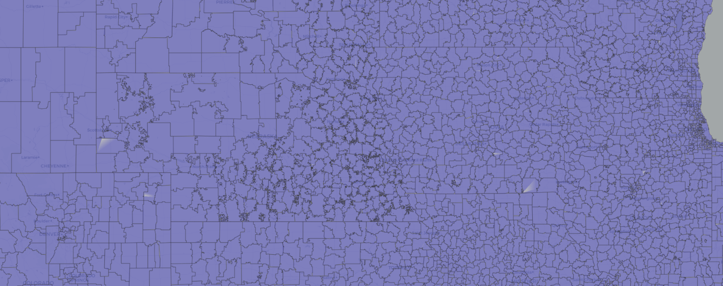
Several weeks ago, I came across the tweet below from Kyle Walker who shared an example of how to pull a large amount of geospatial data with a few lines of code using the tigris package that he developed. The school district data that he showed in his example stood out for the complex boundaries of some states (i.e., Nebraska) compared to bordering states. In this post, I’m going to go through a brief exploration of American public school district boundaries using the tigris and sf packages, along with a tidyverse-style workflow, and identify how some districts are drawn much more differently than others.

Whoa, Nebraska really stands out with all the school district exclaves. pic.twitter.com/3hX9BMYPf2

— Josh Fangmeier (@joshfangmeier) August 4, 2022

Load school district data

To retrieve the school district boundary data, we will use the tigris package, which downloads and loads TIGER/Line shapefiles from the US Census bureau. The school_districts function in tigris downloads school district data, which the Census bureau collects from state education officials. For our analysis, we will use data on unified and elementary districts as of 2021, which combined gives us very good coverage.

library(tidyverse)
library(sf)
library(tigris)
library(mapview)
library(rmapshaper)
library(nngeo)
library(gt)
library(gtExtras)
library(measurements)

Not all states have elementary districts, so we use the safely workflow from the purrr package to keep states that do.

sch_uni_sf <- 
  map_dfr(
    c(state.abb, "DC"),
    ~school_districts(
      state = .x,
      type = "unified",
      year = 2021,
      progress_bar = F
    )
  )

safe_school_districts <- safely(school_districts)

sch_ele_sf <- 
  map(
    c(state.abb, "DC"),
    ~safe_school_districts(
      state = .x,
      type = "elementary",
      year = 2021,
      progress_bar = F
    )
  ) %>% 
  map("result") %>% 
  compact() %>% 
  bind_rows()

fips <- 
  tigris::fips_codes %>% 
  select(
    STATEFP = state_code,
    STUSPS = state,
    STATE_NAME = state_name) %>% 
  distinct()

sch_sf <- 
  bind_rows(
    sch_uni_sf,
    sch_ele_sf
    ) %>% 
  inner_join(
    fips,
    by = "STATEFP"
  )

glimpse(sch_sf)
## Rows: 12,805
## Columns: 18
## $ STATEFP    <chr> "01", "01", "01", "01", "01", "01", "01", "01", "01", "01",~
## $ UNSDLEA    <chr> "00001", "00003", "00005", "00006", "00007", "00008", "0001~
## $ GEOID      <chr> "0100001", "0100003", "0100005", "0100006", "0100007", "010~
## $ NAME       <chr> "Fort Rucker School District", "Maxwell AFB School District~
## $ LSAD       <chr> "00", "00", "00", "00", "00", "00", "00", "00", "00", "00",~
## $ LOGRADE    <chr> "KG", "KG", "KG", "PK", "KG", "PK", "KG", "PK", "KG", "KG",~
## $ HIGRADE    <chr> "12", "12", "12", "12", "12", "12", "12", "12", "12", "12",~
## $ MTFCC      <chr> "G5420", "G5420", "G5420", "G5420", "G5420", "G5420", "G542~
## $ SDTYP      <chr> "B", "B", NA, NA, NA, NA, NA, NA, NA, NA, NA, NA, NA, NA, N~
## $ FUNCSTAT   <chr> "E", "E", "E", "E", "E", "E", "E", "E", "E", "E", "E", "E",~
## $ ALAND      <dbl> 232948114, 8697481, 69770754, 1265301295, 124178343, 786179~
## $ AWATER     <dbl> 2801707, 372428, 258708, 103562192, 2505910, 339435, 601265~
## $ INTPTLAT   <chr> "+31.4097368", "+32.3809438", "+34.2631303", "+34.3821918",~
## $ INTPTLON   <chr> "-085.7458071", "-086.3637490", "-086.2106600", "-086.30505~
## $ ELSDLEA    <chr> NA, NA, NA, NA, NA, NA, NA, NA, NA, NA, NA, NA, NA, NA, NA,~
## $ STUSPS     <chr> "AL", "AL", "AL", "AL", "AL", "AL", "AL", "AL", "AL", "AL",~
## $ STATE_NAME <chr> "Alabama", "Alabama", "Alabama", "Alabama", "Alabama", "Ala~
## $ geometry   <MULTIPOLYGON [°]> MULTIPOLYGON (((-85.86572 3..., MULTIPOLYGON (~

We can see that resulting data frame includes a geometry column of the ‘MULTIPOLYGON’ class. This means that each row (school district) may contains more than one land parcel.

To preview the school district boundaries, we can create a simplified map with ms_simplify from the rmapshaper package and view it with the mapView function.

sch_simp <- 
  ms_simplify(
    sch_sf, 
    sys = T, 
    sys_mem = 4)

m <- mapview(sch_simp)
m

m@map %>% 
  leaflet::setView(-96, 39, zoom = 4)