Posit Table Contest Submission: Amtrak System

geospatial
reactable
transportation
Published

December 22, 2022

The following is a repost of my submission in the 2022 Posit Table Contest, which was recognized as one of the runners up in the contest. The original tutorial, stand-alone table, and code repository are available if interested. Huge thanks to the Posit team for hosting this contest.

Table displaying Amtrak routes

Take me directly to the full table in Section 5.

1 Introduction

In this tutorial, I’ll walkthrough the process of developing a table in R using the reactable and reactablefmtr packages and other supplemental packages and functions. The goal is to create a table that describes the Amtrak system, with detail about the routes and the stations. The table displays a route on each row with the included stations along that route available as expandable details. To help visualize the stations and routes, the table includes embedded graphics generated by ggplot2.

1.1 Load packages and prepared data

The data used for this table comes from multiple sources including the US Department of Transportation, Wikipedia, and TrainWeb.org. The data preparation script and the generated data files are available in the Github repository.

Show the code
library(tidyverse)
library(reactable)
library(reactablefmtr)
library(sf)
library(lwgeom)
library(viridis)
library(ggbump)
library(tigris)
library(htmltools)

stations_df <- read_rds(here::here("data", "amtrak", "stations.rds"))
routes_df <- read_rds(here::here("data", "amtrak", "routes.rds"))
riders_df <- read_rds(here::here("data", "amtrak", "riders.rds"))

1.2 Prepare state/provincial boundary data

To generate maps of the United States and Canada, the tigris package provides US Census Bureau boundaries of states and the canadianmaps package includes data on provinces.

Show the code
states_sf <- 
  states(cb = T, progress_bar = F) %>% 
  filter(
    STUSPS %in% c(state.abb, "DC"),
    !STUSPS %in% c("HI", "AK")) %>% 
  select(ST_PROV = STUSPS)

sf_use_s2(FALSE)

provs_sf <- 
  canadianmaps::PROV %>% 
  st_make_valid() %>% 
  st_transform(crs = st_crs(states_sf)) %>% 
  select(ST_PROV = PT)

states_prov_sf <- 
  bind_rows(
    states_sf,
    provs_sf
  )

2 Routes

We can see that the routes data set includes all 43 active Amtrak routes and 9 variables, such as the beginning and ending cities, passenger volume in fiscal year 2021, length, duration, and which kind of train cars the route includes.

Show the code
glimpse(routes_df)
Rows: 43
Columns: 9
$ name              <chr> "Northeast Regional", "Acela", "Pacific Surfliner", …
$ route             <chr> "Boston/Springfield-New York-Washington-Norfolk/Newp…
$ daily_round_trips <chr> "18 (weekday), 15 (weekend)", "16 (weekday), 4 (Sat)…
$ fy2021_passengers <dbl> 3960000, 897600, 841000, 613200, 434100, 394300, 354…
$ route_miles       <chr> "644 (Newport News);679 (Norfolk);682 (Roanoke)", "4…
$ time              <chr> "14h 0m", "6h 30m ", "8h 30m", "8h 25m", "6h 15m (Oa…
$ url               <chr> "https://en.wikipedia.org/wiki/Northeast_Regional", …
$ cars              <chr> "Business, Coach, Cafe", "First Class, Business, Caf…
$ geometry          <GEOMETRY [°]> MULTILINESTRING ((-77.47296..., MULTILINEST…

2.1 Generate route maps for the table

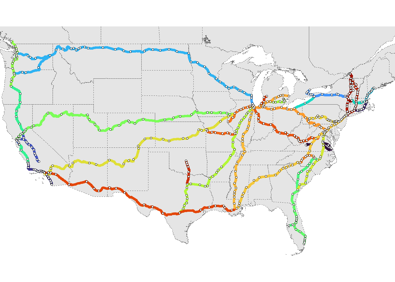
The route data set also includes route geometry that we can use for geospatial analysis. In the code below, we create the routes and routes_map dataframes which will be used for the table. routes_map is generated using the route_map_fcn function which generates a ggplot2 map graphic using the route, station, and state/province geometries. We also generated a separate map graphic for the table header (rendered below).

Show the code
routes <- 
  routes_df %>% 
  mutate(
    map_plot = NA
  ) %>% 
  arrange(desc(fy2021_passengers)) %>% 
  bind_cols(
    route_color = turbo(nrow(routes_df))
  ) %>% 
  st_drop_geometry() %>% 
  arrange(name)

route_map_fcn <- function(route_sf, stations_sf, states_sf) {
  
  route_mer <- st_set_geometry(route_sf, route_sf$geometry) %>% st_transform(crs = 3857)
  stations_mer <- stations_sf %>% st_transform(crs = 3857)
  states_mer <- states_sf %>% st_transform(crs = 3857)
  route_circle <- st_minimum_bounding_circle(st_simplify(route_mer, dTolerance = 1000))
  route_bbox <- st_bbox(route_circle) %>% st_as_sfc()
  route_name <- route_sf$name
  
  gg <- 
    (ggplot() +
       geom_sf(data = states_mer, linetype = "dashed", fill = "gray90", size = 0.25) +
       geom_sf(data = route_mer, aes(color = route_color), size = 1.75) +
       geom_sf(data = stations_mer, shape = 21, size = 1.25, fill = 'white', stroke = 0.5) +
       scale_color_identity() +
       coord_sf(
         xlim = st_coordinates(route_bbox)[c(1,2),1], # min & max of x values
         ylim = st_coordinates(route_bbox)[c(2,3),2]) + # min & max of y values
       theme_void() +
       theme(
         legend.position = 'none',
         panel.background = element_rect(fill = 'transparent', color = NA),
         plot.background = element_rect(fill = 'transparent', color = NA)))
  
  result <- tibble(route = route_name, plot = list(gg))
  
  return(result)
}

routes_stations_sf <- 
  stations_df %>% 
  filter(route != "Winter Park Express") %>% 
  group_by(route) %>% 
  summarize() %>% 
  ungroup() %>% 
  arrange(route)

routes_map_sf <-
  routes %>%
  inner_join(
    routes_df %>% select(name, geometry),
    by = "name") %>%
  select(
    name,
    route_color,
    geometry) %>% 
  arrange(name)

routes_map_sf <- st_set_geometry(routes_map_sf, routes_map_sf$geometry)

routes_map <-
  map2_dfr(
    .x = group_split(routes_map_sf, name),
    .y = group_split(routes_stations_sf, route),
    .f = ~route_map_fcn(route_sf = .x, stations_sf = .y, states_sf = states_prov_sf))

state_route_map <- 
  ggplot() +
  geom_sf(data = states_prov_sf, linetype = "dashed", fill = "gray90", linewidth = 0.25) +
  geom_sf(data = routes_map_sf, aes(color = route_color), linewidth = 1.5, alpha = 1.0) +
  geom_sf(data = routes_stations_sf, shape = 21, size = 1, fill = 'white', stroke = 0.50) +
  coord_sf(xlim = c(-124.763, -66.949), ylim = c(24.523, 51), expand = FALSE) +
  scale_color_identity() +
  theme_void() +
  theme(legend.position = 'none')

state_route_map

2.2 Create functions to generate icons representing available train cars

Each of the routes uses one or more different types of train cars (dining, coach, etc.). To display this information, we use the function below to replace the word descriptions with icons representing whether each type of train car is present for the route.

Show the code
icons <- function(icon, color, size = 30, empty = FALSE) {
  
  fill_color <- grDevices::adjustcolor(color, alpha.f = 1.0)
  empty_color <- grDevices::adjustcolor(color, alpha.f = 0.3)
  
  htmltools::tagAppendAttributes(
    shiny::icon(icon),
    style = paste0("font-size:", size, "px", "; color:", if (empty) empty_color else fill_color),
    "aria-hidden" = "true"
    )
}

train_icons <- function(vals) {
  
  if(is.na(vals)) {
    
    coach <- span(icons("train", "gray10", empty = T), title = "Coach Not Available", style = "margin: 5px;")
    diner <- span(icons("utensils", "gray10", empty = T), title = "Diner/Cafe Not Available", style = "margin: 5px;")
    sleeper <- span(icons("bed", "gray10", empty = T), title = "Sleeper Not Available", style = "margin: 5px;")
    business <- span(icons("briefcase", "gray10", empty = T), title = "Business Not Available", style = "margin: 5px;")
    first_class <- span(icons("money-check-dollar", "gray10", empty = T), title = "First Class Not Available", style = "margin: 5px;")
    auto <- span(icons("car-side", "gray10", empty = T), title = "Auto Transport Not Available", style = "margin: 5px;")
    
  } else {
  
    if (str_detect(vals, "Coach")) {
      coach <- span(icons("chair", "gray10", empty = F), title = "Coach Available", style = "margin: 5px;")
    } else {
      coach <- span(icons("chair", "gray10", empty = T), title = "Coach Not Available", style = "margin: 5px;")
    }
    if (str_detect(vals, "Dinner|Dinette|Cafe|Bistro")) {
      diner <- span(icons("utensils", "gray10", empty = F), title = "Diner/Cafe Available", style = "margin: 5px;")
    } else {
      diner <- span(icons("utensils", "gray10", empty = T), title = "Diner/Cafe Not Available", style = "margin: 5px;")
    }
    if (str_detect(vals, "Sleeper")) {
      sleeper <- span(icons("bed", "gray10", empty = F), title = "Sleeper Available", style = "margin: 5px;")
    } else {
      sleeper <- span(icons("bed", "gray10", empty = T), title = "Sleeper Not Available", style = "margin: 5px;")
    }
    if (str_detect(vals, "Business")) {
      business <- span(icons("briefcase", "gray10", empty = F), title = "Business Available", style = "margin: 5px;")
    } else {
      business <- span(icons("briefcase", "gray10", empty = T), title = "Business Not Available", style = "margin: 5px;")
    }
    if (str_detect(vals, "First Class")) {
      first_class <- span(icons("money-check-dollar", "gray10", empty = F), title = "First Class Available", style = "margin: 5px;")
    } else {
      first_class <- span(icons("money-check-dollar", "gray10", empty = T), title = "First Class Not Available", style = "margin: 5px;")
    }
    if (str_detect(vals, "Auto")) {
      auto <- span(icons("car-side", "gray10", empty = F), title = "Auto Transport Available", style = "margin: 5px;")
    } else {
      auto <- span(icons("car-side", "gray10", empty = T), title = "Auto Transport Not Available", style = "margin: 5px;")
    }
    
  }
  
  div(coach, diner, sleeper, business, first_class, auto)
  
}

2.3 Generate sample routes reactable table

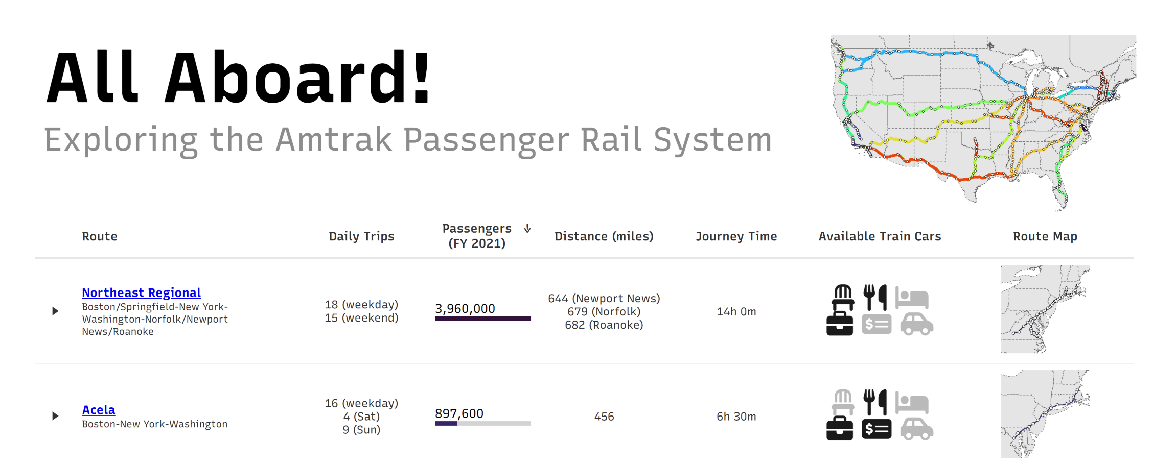
We can now use the route data frames created above to generate a sample reactable table, using the first 5 rows of the routes data. In this table, we create a bar chart of passenger data using reactablefmtr, display the train car icons, include a map graphic, and format the other columns.

Show the code
reactable(
    data = routes %>% slice(1:5),
    highlight = TRUE,
    wrap = TRUE,
    defaultPageSize = 5,
    style = list(
      fontFamily = "Recursive, sans-serif", 
      fontSize = "0.875rem"),
    defaultColDef = colDef(
      vAlign = "center",
      align = "center",
      headerVAlign = "center",
      sortable = FALSE),
    width = 1250,
    defaultSorted = "fy2021_passengers",
    columns = list(
      name = colDef(
        name = "Route",
        align = "left",
        html = TRUE,
        cell = function(value, index) {
          rte <- tags$strong(tags$a(href = as.character(routes[index, "url"]), target = "_blank", value))
          rte_cities <- as.character(routes[index, "route"])
          cities <- div(style = list(float = "left", fontSize = "0.7rem"), rte_cities)
          if (value == "Adirondack") {
            sup <- tags$sup("*")
          } else if (value %in% c("Berkshire Flyer", "Valley Flyer")) {
            sup <- tags$sup("**") 
          } else {
            sup <- NULL
          }
          tagList(rte, sup, tags$br(), cities)
        },
        width = 250,
        sortable = TRUE
      ),
      daily_round_trips = colDef(
        name = "Daily Trips",
        html = TRUE,
        cell = function(value) {
          str_replace_all(value, "\\,", "<br>")
        },
        width = 150,
        style = list(fontSize = "0.8rem")
      ),
      fy2021_passengers = colDef(
        name = "Passengers (FY 2021)",
        defaultSortOrder = "desc",
        cell = data_bars(
          routes,
          fill_color_ref = "route_color",
          text_position = "above",
          number_fmt = scales::comma,
          background = "lightgray"
        ),
        width = 125,
        sortable = TRUE
      ),
      route_miles = colDef(
        name = "Distance (miles)",
        html = TRUE,
        cell = function(value) {
          str_replace_all(value, "\\;", "<br>")
        },
        width = 150,
        style = list(fontSize = "0.8rem")
      ),
      time = colDef(
        name = "Journey Time",
        html = TRUE,
        cell = function(value) {
          str_replace_all(value, "\\;", "<br>")
        },
        width = 150,
        style = list(fontSize = "0.8rem")
      ),
      cars = colDef(
        name = "Available Train Cars",
        cell = function(value) {
          train_icons(value)
        },
        width = 175
      ),
      map_plot = colDef(
        name = "Route Map",
        cell = function(value, index){
          htmltools::plotTag(
            routes_map$plot[[index]],
            alt = 'plots',
            height = 100,
            width = 100,
            deviceArgs = list(bg = 'transparent'))
          },
        width = 200
      ),
      route = colDef(show = FALSE),
      url = colDef(show = FALSE),
      route_color = colDef(show = FALSE)
    )
) %>% 
  div(
    .,
    style = css(
    'text-align' = 'center')
  )

3 Stations and ridership

The stations data set includes all 876 active Amtrak route/station combinations and variables such as the station location, what other routes the station serves, when the station opened, and what type of station it is. The data also includes a variable indicating what type of station junction it is along the route (beginning, middle, split, end, etc.).

The ridership data includes ridership by station from fiscal year 2005 to 2021.

Show the code
glimpse(stations_df)
Rows: 876
Columns: 13
$ route             <chr> "Acela", "Acela", "Acela", "Acela", "Acela", "Acela"…
$ stop_num          <int> 1, 2, 3, 4, 5, 6, 7, 8, 9, 10, 11, 12, 13, 14, 15, 1…
$ junction_type     <chr> "sta", "cont", "cont", "cont", "cont", "cont", "cont…
$ station_name      <chr> "Boston South (BOS)", "Boston Back Bay (BBY)", "West…
$ station_abbr      <chr> "BOS", "BBY", "RTE", "PVD", "NLC", "NHV", "STM", "NY…
$ state_or_province <chr> "MA", "MA", "MA", "RI", "CT", "CT", "CT", "NY", "NJ"…
$ country           <chr> "US", "US", "US", "US", "US", "US", "US", "US", "US"…
$ station_routes    <list> <"Lake Shore Limited", "Northeast Regional">, <"Lak…
$ other_routes      <chr> "Lake Shore Limited; Northeast Regional", "Lake Shor…
$ opened            <dbl> 1899, 1860, 1953, 1986, 1848, 1920, 1849, 1910, 1935…
$ station_type      <chr> "Station Building (with waiting room)", "Station Bui…
$ url               <chr> "https://en.wikipedia.org/wiki/South_Station", "http…
$ geometry          <POINT [°]> POINT (-71.0553 42.35232), POINT (-71.07583 42…
Show the code
glimpse(riders_df)
Rows: 8,908
Columns: 3
$ station_abbr <chr> "ABE", "ABE", "ABE", "ABE", "ABE", "ABE", "ABE", "ABE", "…
$ year         <int> 2005, 2006, 2007, 2008, 2009, 2010, 2011, 2012, 2013, 201…
$ riders       <dbl> 23438, 18008, 38702, 45052, 44495, 41114, 39878, 43987, 4…

3.1 Join station and ridership data and create subway-style route diagrams

Since the stations in a route may be along different branches, it’s helpful to display the data using a route diagram. Some Wikipedia articles (see example) include helpful subway-style route diagrams to display different types of junctions. The route_diagram_fcn below generate specific diagram for each type of junction in ggplot2 in the stations_diag dataframe, which will be used with the stations dataframe in the table.

Show the code
route_diagram_fcn <- function(node_type, line_color) {
  
  if (node_type == "1-2_split") {
    lines_df <-
      tibble(
        x = c(-1, 0, 0, 0),
        y = c(-3, 0, -3, 3),
        group = c(1, 1, 1, 1)
      )
  } else if (node_type == "1-2_split_aft") {
    lines_df <-
      tibble(
        x = c(-1, 0, 0, 0),
        y = c(-3, -1.5, -3, 3),
        group = c(1, 1, 1, 1)
      )
  } else if (node_type == "2-1_comb") {
    lines_df <-
      tibble(
        x = c(-1, 0, 0, 0),
        y = c(3, 0,-3, 3),
        group = c(1, 1, 1, 1)
      )
  } else if (node_type == "sta") {
    lines_df <-
      tibble(x = c(0, 0),
             y = c(0, -3),
             group = c(1, 1))
  } else if (node_type == "beg_bypass") {
    lines_df <-
      tibble(x = c(-1, 0, 0),
             y = c(-3, 0, 3),
             group = c(1, 1, 1))
  } else if (node_type == "cont") {
    lines_df <-
      tibble(x = c(0, 0, 0),
             y = c(0, 3,-3),
             group = c(1, 1, 1))
  } else if (node_type == "cont_aft_bypass") {
    lines_df <-
      tibble(x = c(-1, 0, 0),
             y = c(3, 0, -3),
             group = c(1, 1, 1))
  } else if (node_type == "cont_w_bypass") {
    lines_df <-
      tibble(x = c(0, 0, -1, -1),
             y = c(3, -3, 3, -3),
             group = c(1, 1, 2, 2))
  } else if (node_type == "end") {
    lines_df <-
      tibble(x = c(0, 0),
             y = c(0, 3),
             group = c(1, 1))
  } else if (node_type == "end_w_bypass") {
    lines_df <-
      tibble(x = c(0, 0, -1, -1),
             y = c(0, 3, 3, -3),
             group = c(1, 1, 2, 2))
  } else if (node_type == "sta_w_bypass") {
    lines_df <-
      tibble(x = c(0, 0, -1, -1),
             y = c(0, -3, 3, -3),
             group = c(1, 1, 2, 2))
  }
  
  pts_df <- 
  tibble(
    x = 0,
    y = 0
  )
  
  ggplot() +
    geom_bump(
      data = lines_df, 
      aes(x, y, group = group), 
      linewidth = 4, 
      color = line_color, 
      direction = "y") +
    geom_point(
      data = pts_df, 
      aes(x, y), 
      shape = 21, 
      size = 10, 
      stroke = 2,
      color = "gray20", 
      fill = "white") +
    scale_color_identity() +
    scale_x_continuous(expand = c(0, 0)) + 
    scale_y_continuous(expand = c(0, 0)) +
    coord_cartesian(xlim = c(-2, 2), ylim = c(-3, 3)) +
    theme_void()
}

riders <- 
  riders_df %>% 
  separate_rows(station_abbr, sep = "\\/") %>% 
  arrange(year) %>% 
  group_by(station_abbr) %>% 
  summarize(riders = list(riders)) %>% 
  ungroup()

stations <- 
  stations_df %>% 
  st_drop_geometry() %>% 
  inner_join(
    routes %>% select(route = name, route_color),
    by = "route"
  ) %>% 
  inner_join(
    tibble(
      state_or_province = c(state.abb, "DC", "ON", "QC", "BC"),
      st_prov_name = c(state.name, "District of Columbia", "Ontario", "Quebec", "British Columbia")
    ),
    by = "state_or_province"
  ) %>% 
  left_join(
    riders, by = "station_abbr"
  ) %>% 
  select(-station_abbr) %>% 
  transmute(
    route,
    route_color,
    junction_type,
    station_name,
    url,
    st_prov_name,
    country,
    riders = modify_if(riders, ~is.null(.), ~rep(NA_real_, 17)),
    opened,
    station_type,
    station_routes = map(station_routes, ~str_subset(.x, "Winter Park Express", negate = T)),
    other_routes = modify_if(station_routes, ~length(.) == 0, ~NA_character_),
    other_routes = map_chr(other_routes, ~glue::glue_collapse(.x, sep = "; "))
  )

stations_diag <-
  stations %>%
  select(route, station_name, junction_type, route_color) %>%
  mutate(PLOT = map2(junction_type, route_color, ~route_diagram_fcn(node_type = .x, line_color = .y)))

3.2 Generate sample stations reactable table

Similar to the routes table above, we can use the stations data frames created above to generate a sample reactable table, using the stations on the Northeast Regional route. In this table, we embed the route diagram for the station, create a sparkline chart of passenger data using reactablefmtr, display the connecting routes using a details breakout, and format the other columns.

Show the code
stat_data <- stations %>% filter(route == "Northeast Regional")
stat_route_color <- stat_data %>% pull(route_color) %>% unique()
stat_plot <- inner_join(stations_diag, stat_data, by = c("route", "station_name"))
      
reactable(
  stat_data,
  outlined = FALSE,
  theme = reactableTheme(
    cellPadding = "0px 6px",
    style = list(".rt-tr-details" = list("text-align" = "right"))
  ),
  style = list(fontFamily = "Recursive, sans-serif",
               fontSize = "0.875rem"),
  defaultPageSize = nrow(stat_data),
  defaultColDef = colDef(
    vAlign = "center",
    align = "center",
    headerVAlign = "center"
  ),
  width = 1250,
  sortable = FALSE,
  columns = list(
    junction_type = colDef(
      name = "",
      resizable = FALSE,
      align = "left",
      cell = function(value, index) {
        htmltools::plotTag(
          stat_plot$PLOT[[index]],
          alt = 'plots',
          height = 100,
          width = 100
        )
      },
      width = 100
    ),
    station_name = colDef(
      name = "Station",
      resizable = TRUE,
      align = "left",
      cell = function(value, index) {
        stat_url <-
          tags$a(href = as.character(stat_data[index, "url"]), target = "_blank", value)
        state <-
          as.character(stat_data[index, "st_prov_name"])
        country <- as.character(stat_data[index, "country"])
        flag_url <- paste0(
          "https://raw.githubusercontent.com/catamphetamine/country-flag-icons/master/flags/1x1/",
          country,
          ".svg"
        )
        flag_img <-
          image <-
          img(src = flag_url, style = "width:45px;height:15px;", alt = country)
        state_div <-
          div(style = list(float = "left", fontSize = "0.7rem"),)
        tagList(stat_url, tags$br(), state, flag_img)
      },
      minWidth = 250
    ),
    riders = colDef(
      name = "Station Ridership (FY 2005-2021)",
      cell = react_sparkline(
        stat_data,
        decimals = 0,
        tooltip_type = 2,
        height = 100,
        show_area = TRUE,
        line_width = 2,
        area_color_ref = "route_color",
        area_opacity = 0.5,
        margin = margin(10, 5, 10, 0)
      ),
      width = 450
    ),
    opened = colDef(
      name = "Year Opened (Rebuilt)",
      cell = color_tiles(
        data = stat_data,
        colors = stat_route_color %>% shades::saturation(seq(0.2, 1, 0.2)) %>% as.character(),
        opacity = 0.7,
        bold_text = FALSE,
        box_shadow = FALSE
      ),
      width = 150
    ),
    station_type = colDef(
      name = "Station Type",
      cell = function(value, index) {
        if (is.na(value)) {
          station_icon <- 'train'
        } else if (value == "Station Building (with waiting room)") {
          station_icon <- 'building-user'
        } else if (value == "Platform with Shelter") {
          station_icon <- 'people-roof'
        } else {
          station_icon <- 'train'
        }
        span(icons(station_icon, "gray10", empty = F),
             title = value,
             style = "margin: 5px;")
      },
      width = 125
    ),
    station_routes = colDef(
      name = "Connecting Routes",
      html = TRUE,
      cell = function(value, index) {
        if (length(value) == 0) {
          "NA"
        } else {
          paste0(length(value), " routes")
        }
      },
      details = function(index) {
        if (length(stat_data$station_routes[index][[1]]) > 0) {
          connections <- stat_data$other_routes[index]
          paste0("Connecting to: ", connections)
        }
      },
      width = 125
    ),
    route = colDef(show = FALSE),
    stop_num = colDef(show = FALSE),
    url = colDef(show = FALSE),
    state_or_province = colDef(show = FALSE),
    country = colDef(show = FALSE),
    other_routes = colDef(show = FALSE),
    route_color = colDef(show = FALSE),
    st_prov_name = colDef(show = FALSE)
  )
) %>% 
  div(
    .,
    style = css(
    'text-align' = 'center')
  )

4 Generate nested reactable table including routes and stations

Finally, we can bring together the routes and stations data into one reactable table. After creating the amtrak_table object, we add headers and footers using the prependContent and appendContent functions in the htmlwidgets package. The header includes the map graphic of the whole Amtrak system as well as the title and subtitle. The footer includes footnotes and source information.

Show the code
amtrak_table <- 
  reactable(
    data = routes,
    highlight = TRUE,
    wrap = TRUE,
    defaultPageSize = nrow(routes),
    style = list(
      fontFamily = "Recursive, sans-serif", 
      fontSize = "0.875rem"),
    defaultColDef = colDef(
      vAlign = "center",
      align = "center",
      headerVAlign = "center",
      sortable = FALSE),
    width = 1250,
    defaultSorted = "fy2021_passengers",
    columns = list(
      name = colDef(
        name = "Route",
        align = "left",
        html = TRUE,
        cell = function(value, index) {
          rte <- tags$strong(tags$a(href = as.character(routes[index, "url"]), target = "_blank", value))
          rte_cities <- as.character(routes[index, "route"])
          cities <- div(style = list(float = "left", fontSize = "0.7rem"), rte_cities)
          if (value == "Adirondack") {
            sup <- tags$sup("*")
          } else if (value %in% c("Berkshire Flyer", "Valley Flyer")) {
            sup <- tags$sup("**") 
          } else {
            sup <- NULL
          }
          tagList(rte, sup, tags$br(), cities)
        },
        width = 250,
        sortable = TRUE
      ),
      daily_round_trips = colDef(
        name = "Daily Trips",
        html = TRUE,
        cell = function(value) {
          str_replace_all(value, "\\,", "<br>")
        },
        width = 150,
        style = list(fontSize = "0.8rem")
      ),
      fy2021_passengers = colDef(
        name = "Passengers (FY 2021)",
        defaultSortOrder = "desc",
        cell = data_bars(
          routes,
          fill_color_ref = "route_color",
          text_position = "above",
          number_fmt = scales::comma,
          background = "lightgray"
        ),
        width = 125,
        sortable = TRUE
      ),
      route_miles = colDef(
        name = "Distance (miles)",
        html = TRUE,
        cell = function(value) {
          str_replace_all(value, "\\;", "<br>")
        },
        width = 150,
        style = list(fontSize = "0.8rem")
      ),
      time = colDef(
        name = "Journey Time",
        html = TRUE,
        cell = function(value) {
          str_replace_all(value, "\\;", "<br>")
        },
        width = 150,
        style = list(fontSize = "0.8rem")
      ),
      cars = colDef(
        name = "Available Train Cars",
        cell = function(value) {
          train_icons(value)
        },
        width = 175
      ),
      map_plot = colDef(
        name = "Route Map",
        cell = function(value, index){
          htmltools::plotTag(
            routes_map$plot[[index]],
            alt = 'plots',
            height = 100,
            width = 100,
            deviceArgs = list(bg = 'transparent'))
          },
        width = 200
      ),
      route = colDef(show = FALSE),
      url = colDef(show = FALSE),
      route_color = colDef(show = FALSE)
    ),
    details = function(index) {
      station_data <- stations[stations$route == routes$name[index], ]
      station_route_color <- station_data %>% pull(route_color) %>% unique()
      htmltools::div(
        style = "padding: 0rem",
        reactable(
          station_data, 
          outlined = FALSE,
          theme = reactableTheme(
            cellPadding = "0px 6px",
            style = list(".rt-tr-details" = list("text-align" = "right"))
          ),
          defaultPageSize = nrow(station_data),
          defaultColDef = colDef(
            vAlign = "center",
            align = "center",
            headerVAlign = "center"),
          width = 1250,
          sortable = FALSE,
          columns = list(
            junction_type = colDef(
              name = "",
              resizable = FALSE,
              align = "left",
              cell = function(value, index){
                station_plot <- inner_join(stations_diag, station_data, by = c("route", "station_name"))
                htmltools::plotTag(
                  station_plot$PLOT[[index]],
                  alt = 'plots',
                  height = 100,
                  width = 100)
                },
              width = 100
            ),
            station_name = colDef(
              name = "Station",
              resizable = TRUE,
              align = "left",
              cell = function(value, index) {
                stat_url <- tags$a(href = as.character(station_data[index, "url"]), target = "_blank", value)
                state <- as.character(station_data[index, "st_prov_name"])
                country <- as.character(station_data[index, "country"])
                flag_url <- paste0(
                  "https://raw.githubusercontent.com/catamphetamine/country-flag-icons/master/flags/1x1/", 
                  country, ".svg")
                flag_img <- image <- img(src = flag_url, style = "width:45px;height:15px;", alt = country)
                state_div <- div(style = list(float = "left", fontSize = "0.7rem"), )
                tagList(stat_url, tags$br(), state, flag_img)
                },
              minWidth = 250
              ),
            riders = colDef(
              name = "Station Ridership (FY 2005-2021)",
              cell = react_sparkline(
                station_data,
                decimals = 0,
                tooltip_type = 2,
                height = 100,
                show_area = TRUE,
                line_width = 2,
                area_color_ref = "route_color",
                area_opacity = 0.5,
                margin = margin(10, 5, 10, 0)
                ),
              width = 450),
            opened = colDef(
              name = "Year Opened (Rebuilt)",
               cell = color_tiles(
                 data = station_data,
                 colors = station_route_color %>% shades::saturation(seq(0.2, 1, 0.2)) %>% as.character(),
                 opacity = 0.7,
                 bold_text = FALSE,
                 box_shadow = FALSE
                 ),
              width = 150
              ),
            station_type = colDef(
              name = "Station Type",
              cell = function(value, index) {
                if (is.na(value)) {
                  station_icon <- 'train'
                } else if (value == "Station Building (with waiting room)") {
                  station_icon <- 'building-user'
                } else if (value == "Platform with Shelter") {
                  station_icon <- 'people-roof'
                } else {
                  station_icon <- 'train'
                }
                span(icons(station_icon, "gray10", empty = F), title = value, style = "margin: 5px;")
              },
              width = 125
            ),
            station_routes = colDef(
              name = "Connecting Routes",
              html = TRUE,
              cell = function(value, index) {
                if (length(value) == 0) {
                  "NA"
                } else {
                  paste0(length(value), " routes")
                }
              },
              details = function(index) {
                if (length(station_data$station_routes[index][[1]]) > 0) {
                  connections <- station_data$other_routes[index]
                  paste0("Connecting to: ", connections)
                  }
                },
              width = 125
              ),
            route = colDef(show = FALSE),
            stop_num = colDef(show = FALSE),
            url = colDef(show = FALSE),
            state_or_province = colDef(show = FALSE),
            country = colDef(show = FALSE),
            other_routes = colDef(show = FALSE),
            route_color = colDef(show = FALSE),
            st_prov_name = colDef(show = FALSE)
          ))
      )
      }
  )
Show the code
amtrak_table_final <- 
  amtrak_table %>%
  # add title, subtitle, and map
  htmlwidgets::prependContent(
    tags$div(
      tags$link(
        href = "https://fonts.googleapis.com/css?family=Recursive:400,600,700&display=swap", 
        rel = "stylesheet"),
      tags$div(
        tags$div(
          "All Aboard!", 
        style = css(
          'font-size' = '60pt', 
          'font-weight' = 'bold', 
          'font-family' = 'Recursive', 
          'text-align' = 'left',
          'margin-bottom' = 0,
          'padding-left' = '10px',
          'vertical-align' = 'middle')
        ),
        tags$div(
          "Exploring the Amtrak Passenger Rail System", 
          style = css(
            'font-family' = 'Recursive',
            'margin-bottom' = 0,
            'margin-top' = 0,
            'font-size' = '28pt',
            'text-align' = 'left',
            color = '#8C8C8C',
            'padding-left' = '10px')
          ),
        style = css(width = '70%')
      ),
      tags$div(
        plotTag(
          state_route_map,
          alt = "Map of all Amtrak routes",
          height = 200
          ),
        style = css(width = '30%')),
      style = css(
        width = '1250px',
        display = 'inline-flex'))) %>%
  # add footnotes and source notes
  htmlwidgets::appendContent(
    tags$div(
      tags$link(
        href = "https://fonts.googleapis.com/css?family=Recursive:400,600,700&display=swap", 
        rel = "stylesheet"),
      tags$sup("*"), 
      "Amtrak suspended Adirondack service in July 2021, and no resumption date has been set as of October 2022.",
      tags$br(),
      tags$sup("**"), 
      "Berkshire Flyer seasonal service began in 2022, and Valley Flyer service began in 2019.",
      style = css(
        display = 'inline-block',
        'text-align' = 'left',
        'font-family' = 'Recursive',
        color = 'black', 
        'font-size' = '9pt',
        'border-bottom-style' = 'solid',
        'border-top-style' = 'solid',
        width = '1250px',
        'padding-bottom' = '8px',
        'padding-top' = '8px',
        'padding-left' = '10px',
        'border-color' = '#DADADA')),
    tags$div(
      tags$link(
        href = "https://fonts.googleapis.com/css?family=Roboto:400,600,700&display=swap", 
        rel = "stylesheet"),
      tags$div(
        "Data Sources: Wikipedia, US Dept of Transportation, US Census Bureau, TrainWeb.org, and OpenStreetMaps | ",
        style = css(
          display = 'inline-block', 
          'vertical-align' = 'middle')),
      tags$div(
        shiny::icon("twitter"), 
        style = css(
          display = 'inline-block', 
          'vertical-align' = 'middle')),
      tags$div(
        tags$a("@joshfangmeier", href = "https://twitter.com/joshfangmeier", target = "_blank"),
        style = css(
          display = 'inline-block', 
          'vertical-align' = 'middle')),
      tags$div(
        shiny::icon("github"), 
        style = css(
          display = 'inline-block', 
          'vertical-align' = 'middle')),
      tags$div(
        tags$a("jfangmeier", href = "https://github.com/jfangmeier", target = "_blank"), 
        style = css(
          display = 'inline-block', 
          'vertical-align' = 'middle')),
      style = css(
        'text-align' = 'left',
        'font-family' = 'Roboto', 
        color = '#8C8C8C', 
        'font-size' = '10pt', 
        width = '1250px', 
        'padding-top' = '8px', 
        'padding-left' = '10px',
        display = 'inline-block', 
        'vertical-align' = 'middle')
      )
  )

5 Display the table

All Aboard!
Exploring the Amtrak Passenger Rail System
Map of all Amtrak routes
* Amtrak suspended Adirondack service in July 2021, and no resumption date has been set as of October 2022.
** Berkshire Flyer seasonal service began in 2022, and Valley Flyer service began in 2019.
Data Sources: Wikipedia, US Dept of Transportation, US Census Bureau, TrainWeb.org, and OpenStreetMaps |