library(tidyverse)
library(lubridate)
library(rayshader)
library(raster)
library(sf)
library(mapview)
library(magick)Rayshading the Big Sur Marathon
rayshader
running
marathons
geospatial
Visualizing marathon races
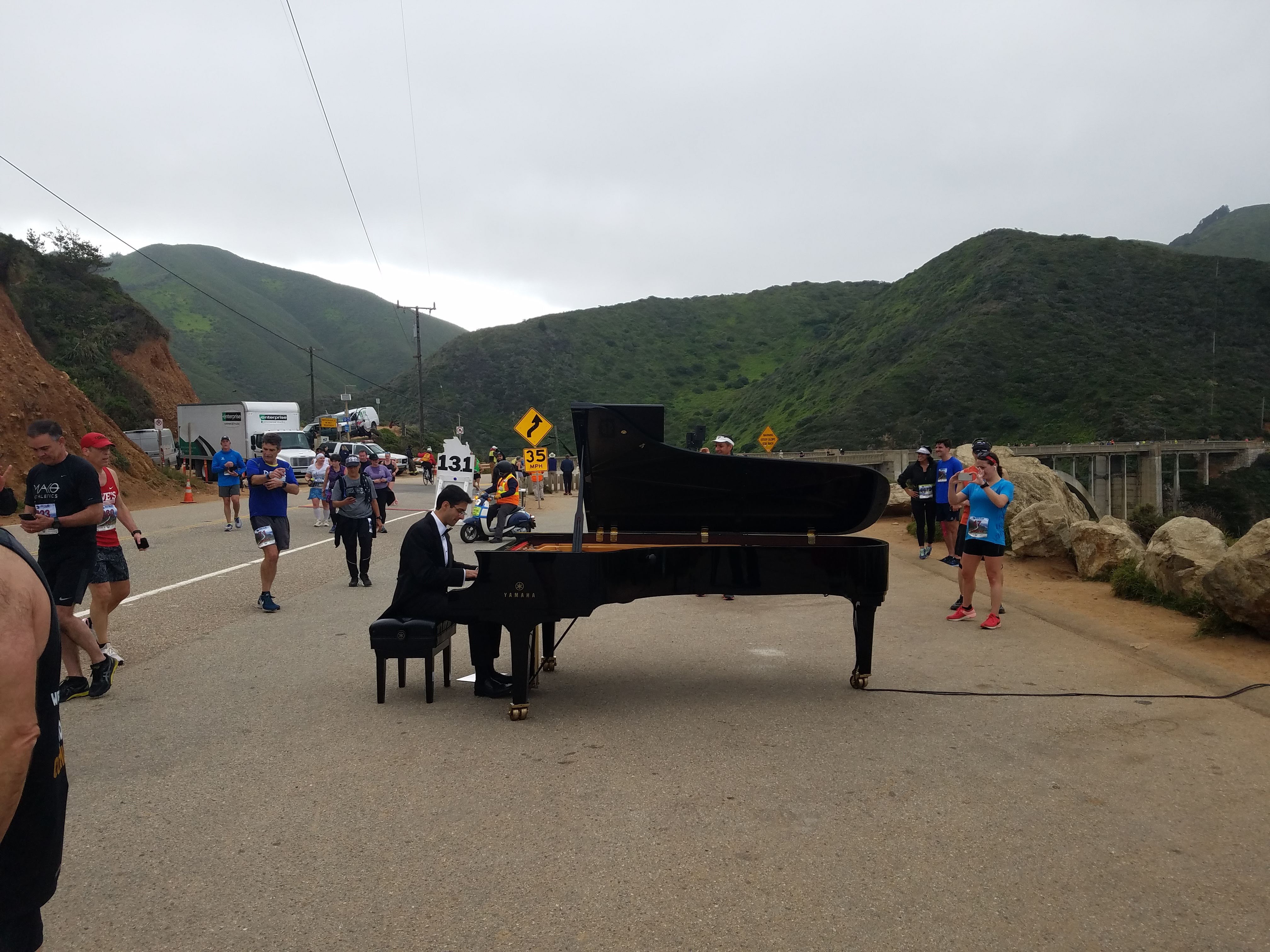
With marathons and other large gatherings canceled or delayed by the COVID-19 pandemic, I’ve been feeling extra nostalgic for past running experiences in some of my favorite places. At the top of the list is the Big Sur Marathon that runs along California State Route 1 from Big Sur Station to Carmel. The course starts near the southern edge of the Redwood forest, rises to the top of Hurricane Point overlooking the Pacific, crosses iconic Bixby Creek Bridge, and passes over numerous hills and turns before reaching the finish. Big Sur is a challenging spring marathon, and while I finished in just over 4 hours in 2019, it was definitely the most difficult race I’ve run. Having a live piano performance at Bixby helped though.
Like other runners, I tracked my progress with GPS, using the RunKeeper app on my phone. This project will use the GPS location data from RunKeeper and visualize the course using the rayshader R package, which can provide a 3-dimensional view of a landscape or other surface. Tyler Morgan-Wall recently posted an excellent guide for combining elevation data with satellite imagery to create 3D renderings of landscapes. Examples from Sebastian Engel-Wolf, Simon Coulombe, and Francois Keck of using animation with rayshader also provided plenty of guidance and inspiration.
Data sources and prep
This project will need the GPS data from RunKeeper, satellite imagery data, and elevation data. Morgan-Wall’s post includes the step-by-step process for downloading the SRTM elevation data and imagery data from USGS. I won’t repeat those steps here, but I’ve pre-downloaded the data for the Big Sur region of California.
Let’s get to it and load the R packages.
First, let’s load the elevation data. I downloaded data for two bordering areas, so I’ll merge them together.
elevation1 <- raster::raster(file.path(path_to_data, "N36W122.hgt"))
elevation2 <- raster::raster(file.path(path_to_data, "N36W123.hgt"))

bigsur_elevation <- raster::merge(elevation1,elevation2)
plot(bigsur_elevation)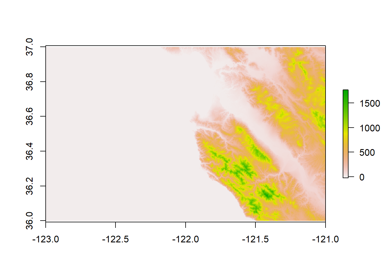
Next, let’s load the satellite data, which comes in three files that are separate layers for the image. After loading the layers, we’ll combine them and apply a color adjustment. It will need more refinement, but the Monterey peninsula is visible.
bigsur_r <- raster::raster(file.path(path_to_data, "LC08_L1TP_044035_20191026_20191030_01_T1_B4.TIF"))
bigsur_g <- raster::raster(file.path(path_to_data, "LC08_L1TP_044035_20191026_20191030_01_T1_B3.TIF"))
bigsur_b <- raster::raster(file.path(path_to_data, "LC08_L1TP_044035_20191026_20191030_01_T1_B2.TIF"))

bigsur_rbg_corrected <- sqrt(raster::stack(bigsur_r, bigsur_g, bigsur_b))
raster::plotRGB(bigsur_rbg_corrected)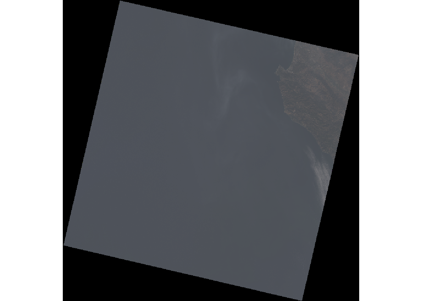
Finally, let’s load the GPS data from RunKeeper, which comes as a GPX file. With a quick view using mapView, we can see the tracked points from the GPS file are in the right locations.
bigsur_gpx <-
  st_read(
    file.path(path_to_data, "RK_gpx_2019-04-28_0643.gpx"),
    layer = "track_points",
    quiet = TRUE
  ) %>%
  dplyr::select(track_seg_point_id, ele, time, geometry)

mapView(bigsur_gpx)
Now that each of the three files are loaded, we need to get them all on the same projection system to get them to play nicely together. In this case, I applied the CRS from the imagery files to the other two files. We will also use the boundaries of the GPS file to crop the dimensions of the other files.
bigsur_extent <-
  bigsur_gpx %>%
  st_transform(., raster::crs(bigsur_r)) %>%
  as_Spatial() %>%
  extent() + 1e4

bigsur_extent
class : Extent
xmin : 590082.3
xmax : 614524.6
ymin : 4007102
ymax : 4049264 rasterOptions(chunksize=1e+06, maxmemory=1e+08)
bigsur_elevation_utm <- raster::projectRaster(bigsur_elevation, crs = crs(bigsur_r), method = "bilinear")
crs(bigsur_elevation_utm)Coordinate Reference System:
Deprecated Proj.4 representation:
+proj=utm +zone=10 +datum=WGS84 +units=m +no_defs
WKT2 2019 representation:
PROJCRS["WGS 84 / UTM zone 10N",
BASEGEOGCRS["WGS 84",
DATUM["World Geodetic System 1984",
ELLIPSOID["WGS 84",6378137,298.257223563,
LENGTHUNIT["metre",1]]],
PRIMEM["Greenwich",0,
ANGLEUNIT["degree",0.0174532925199433]],
ID["EPSG",4326]],
CONVERSION["UTM zone 10N",
METHOD["Transverse Mercator",
ID["EPSG",9807]],
PARAMETER["Latitude of natural origin",0,
ANGLEUNIT["degree",0.0174532925199433],
ID["EPSG",8801]],
PARAMETER["Longitude of natural origin",-123,
ANGLEUNIT["degree",0.0174532925199433],
ID["EPSG",8802]],
PARAMETER["Scale factor at natural origin",0.9996,
SCALEUNIT["unity",1],
ID["EPSG",8805]],
PARAMETER["False easting",500000,
LENGTHUNIT["metre",1],
ID["EPSG",8806]],
PARAMETER["False northing",0,
LENGTHUNIT["metre",1],
ID["EPSG",8807]]],
CS[Cartesian,2],
AXIS["(E)",east,
ORDER[1],
LENGTHUNIT["metre",1]],
AXIS["(N)",north,
ORDER[2],
LENGTHUNIT["metre",1]],
USAGE[
SCOPE["Engineering survey, topographic mapping."],
AREA["Between 126°W and 120°W, northern hemisphere between equator and 84°N, onshore and offshore. Canada - British Columbia (BC); Northwest Territories (NWT); Nunavut; Yukon. United States (USA) - Alaska (AK)."],
BBOX[0,-126,84,-120]],
ID["EPSG",32610]] bigsur_rgb_cropped <- raster::crop(bigsur_rbg_corrected, bigsur_extent)
elevation_cropped <- raster::crop(bigsur_elevation_utm, bigsur_extent)Following Morgan-Wall’s guide, we make a few more adjustments to the imagery data. We now have a nicely cropped image of the marathon course with good contrast and color balance.
names(bigsur_rgb_cropped) <- c("r","g","b")

bigsur_r_cropped <- rayshader::raster_to_matrix(bigsur_rgb_cropped$r)
bigsur_g_cropped <- rayshader::raster_to_matrix(bigsur_rgb_cropped$g)
bigsur_b_cropped <- rayshader::raster_to_matrix(bigsur_rgb_cropped$b)

bigsurel_matrix <- rayshader::raster_to_matrix(elevation_cropped)

bigsur_rgb_array <- array(0,dim=c(nrow(bigsur_r_cropped),ncol(bigsur_r_cropped),3))

bigsur_rgb_array[,,1] <- bigsur_r_cropped/255 #Red layer
bigsur_rgb_array[,,2] <- bigsur_g_cropped/255 #Blue layer
bigsur_rgb_array[,,3] <- bigsur_b_cropped/255 #Green layer

bigsur_rgb_array <- aperm(bigsur_rgb_array, c(2,1,3))

bigsur_rgb_contrast <- scales::rescale(bigsur_rgb_array,to=c(0,1))
plot_map(bigsur_rgb_contrast)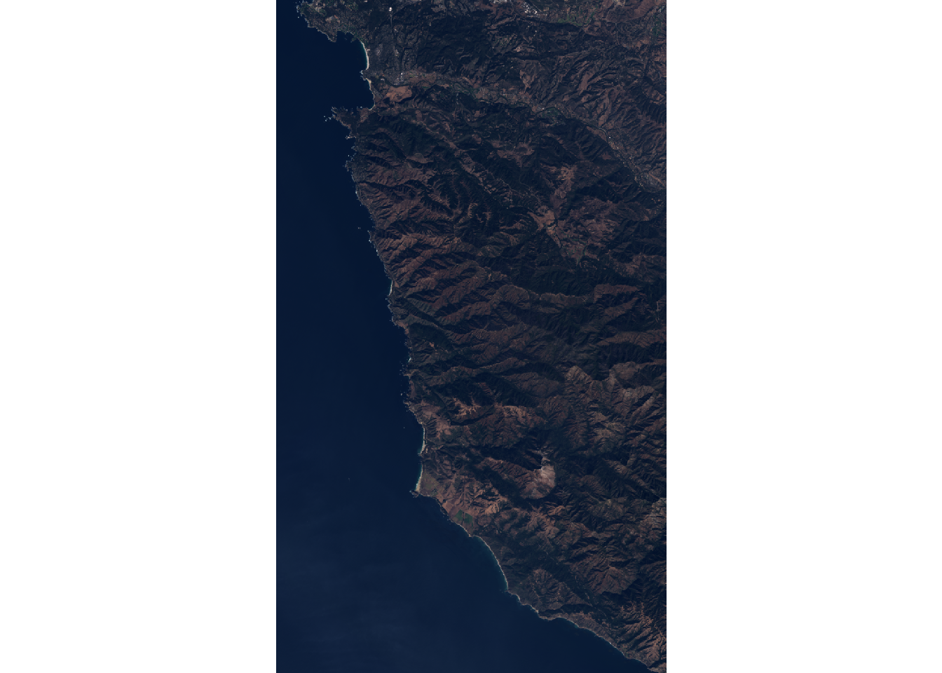
Enhancing and plotting the GPS data
The GPS data only includes elevation, time, and coordinate information right now…
bigsur_gpx %>%
  head(n = 5) %>%
  as_tibble()
# A tibble: 5 x 4
track_seg_point_id ele time geometry
<int> <dbl> <dttm> <POINT [°]>
1 0 92.7 2019-04-28 08:45:22 (-121.781 36.24761)
2 1 92.7 2019-04-28 08:45:22 (-121.781 36.24761)
3 2 92.9 2019-04-28 08:45:33 (-121.7811 36.24765)
4 3 93 2019-04-28 08:45:49 (-121.7812 36.24767)
5 4 93.1 2019-04-28 08:45:53 (-121.7813 36.24771)But we can enhance it to calculate distance between each of the points, along with cumulative distance and time elapsed.
bigsur_gpx_enr <-
  bigsur_gpx %>%
  st_transform(., raster::crs(bigsur_r)) %>%
  mutate(time = as_datetime(time),
         elapsed_time = ifelse(dplyr::row_number() == 1, 0,
                               time - lag(time)),
         distance_from_prior = sf::st_distance(
           geometry,
           lag(geometry),
           by_element = TRUE),
         distance_from_prior = ifelse(is.na(distance_from_prior), 0, distance_from_prior),
         cumul_time = cumsum(elapsed_time),
         cumul_dist = cumsum(distance_from_prior)
  ) %>%
  mutate(row = row_number()) %>%
  as_Spatial() %>%
  data.frame() %>%
  mutate(lon = coords.x1,
         lat = coords.x2,
         dep = ele + 25)
We can also plot the enhanced data to show Hurricane Point near the midpoint of the race (the orange vertical bar), all the times I stopped to take photos, and how my pace variation increased a lot in the last few miles as I started to wear out. The final elapsed time and distance values turned out a little larger than the actual race stats, since I started the GPS before the starting line and after the finish line.
bigsur_gpx_enr %>%
  transmute(cumul_miles = measurements::conv_unit(cumul_dist, "m", "mi"),
         Elevation = measurements::conv_unit(ele, "m", "ft"),
         Pace = elapsed_time / 60 / measurements::conv_unit(distance_from_prior, "m", "mi")) %>%
  pivot_longer(Elevation:Pace, names_to = "measure", values_to = "value") %>%
  ggplot(aes(cumul_miles, value, color = measure)) +
    facet_wrap(~measure, ncol = 1, scale = "free_y") +
  geom_line(size = 1.5) +
  geom_vline(xintercept = 12.2, color = "orange", size = 4, alpha = 0.5) +
  theme_minimal() +
  labs(title = "Big Sur Marathon GPX",
       x = "Distance (miles)",
       y = NULL,
       color = NULL) +
  theme(legend.position = "bottom")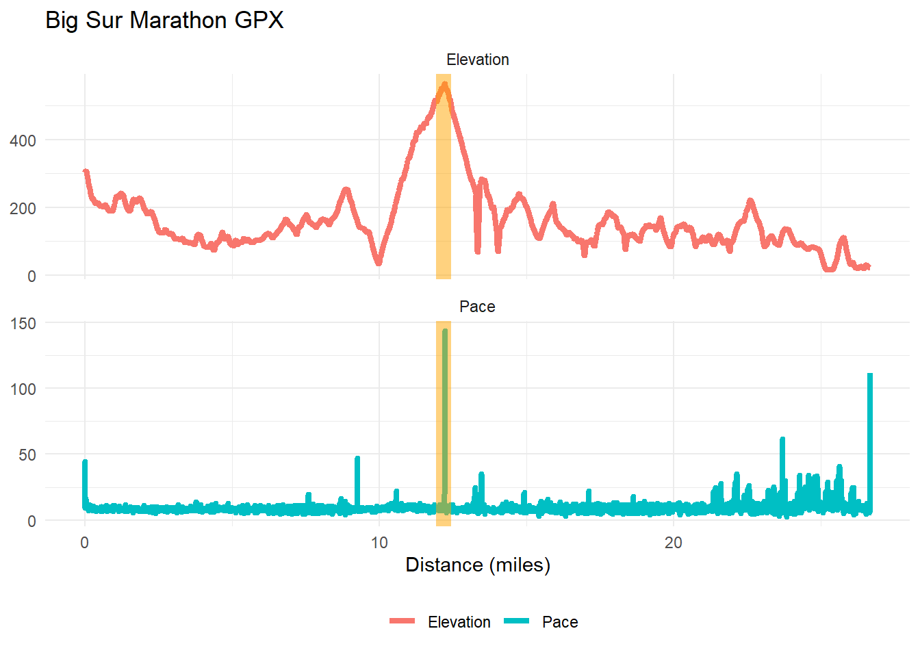
Creating a video animation of the marathon
To put together a video animation of the course, we will need to generate a large number of frames that will later be rendered into a video clip. Each frame will have a specific shot angle and displayed progress on the course.
For generating all the values of the angles, I used the transition_values function from Will Bishop.
transition_values <- function(from, to, steps = 10,
                              one_way = FALSE, type = "cos") {
  if (!(type %in% c("cos", "lin")))
    stop("type must be one of: 'cos', 'lin'")

  range <- c(from, to)
  middle <- mean(range)
  half_width <- diff(range)/2

  # define scaling vector starting at 1 (between 1 to -1)
  if (type == "cos") {
    scaling <- cos(seq(0, 2*pi / ifelse(one_way, 2, 1), length.out = steps))
  } else if (type == "lin") {
    if (one_way) {
      xout <- seq(1, -1, length.out = steps)
    } else {
      xout <- c(seq(1, -1, length.out = floor(steps/2)),
                seq(-1, 1, length.out = ceiling(steps/2)))
    }
    scaling <- approx(x = c(-1, 1), y = c(-1, 1), xout = xout)$y
  }

  middle - half_width * scaling
}
The video will be 24 seconds long at 60 frames per second, so 1,440 frames will need to be created. Here are the values used to create all the angles:
n_frames <- 60 * 24
gpx_rows <- seq(1, nrow(bigsur_gpx_enr), length.out = n_frames) %>% round()
zscale <- 15
thetavalues <- transition_values(from = 280,
                                 to = 130,
                                 steps = n_frames,
                                 one_way = TRUE,
                                 type = "lin")
phivalues <- transition_values(from = 70,
                               to = 20,
                               steps = n_frames,
                               one_way = FALSE,
                               type = "cos")
zoomvalues <- transition_values(from = 0.8,
                                to = 0.3,
                                steps = n_frames,
                                one_way = FALSE,
                                type = "cos")
Another challenge is plotting the GPS coordinates as a 3D line that progresses over time. After trying out a few options, I generated a new add_3d_line function based on Vinay Udyawer’s KUD3D package. This function is essentially a wrapper that takes the coordinate data, calculates point distances, and creates a line using rgl::lines3d.
add_3d_line <-
function(ras,
det,
zscale,
lonlat = FALSE,
col = "red",
alpha = 0.8,
size = 2,
...) {
e <- extent(ras)
cell_size_x <-
raster::pointDistance(c(e@xmin, e@ymin), c(e@xmax, e@ymin), lonlat = lonlat) / ncol(ras)
cell_size_y <-
raster::pointDistance(c(e@xmin, e@ymin), c(e@xmin, e@ymax), lonlat = lonlat) / nrow(ras)
distances_x <-
raster::pointDistance(c(e@xmin, e@ymin), cbind(det$lon, rep(e@ymin, nrow(det))), lonlat = lonlat) / cell_size_x
distances_y <-
raster::pointDistance(c(e@xmin, e@ymin), cbind(rep(e@xmin, nrow(det)), det$lat), lonlat = lonlat) / cell_size_y
rgl::lines3d(
x = distances_y - (nrow(ras)/2),
y = det$dep / zscale,
z = abs(distances_x) - (ncol(ras)/2),
color = col,
alpha = alpha,
lwd = size,
...
)
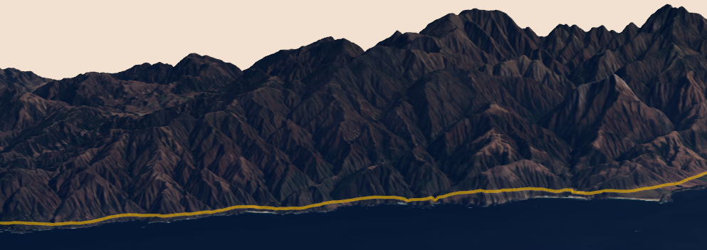
}To bring all the elevation, imagery, and GPS data together, I needed to rotate the imagery and elevation data 90 degrees, so I created a new version of the imagery file and rotated the elevation data using the matlab::rot90 function. I then added labels for the start and finish points of the race by manually finding the coordinates with the best fit.
Within the loop function, I calculated the cumulative distance and elapsed time for each frame and adjusted the camera for the shot angles. Using the new add_3d_line function, I then overlay the 3D path of the race progress over the landscape. After each snapshot is captured, I then remove the path using rgl::rgl.pop to reduce the amount of memory consumed by the creating all the frames.
image_write(image_rotate(image_read(bigsur_rgb_contrast), 90), file.path(path_to_data, "rotated.png"))
overlay_img <- png::readPNG(file.path(path_to_data, "rotated.png"), info = TRUE)

plot_3d(overlay_img,
        matlab::rot90(bigsurel_matrix, k = 1),
        zscale = zscale,
        fov = 0,
        theta = thetavalues[1],
        phi = phivalues[1],
        windowsize = c(1000,800),
        zoom = zoomvalues[1],
        water=FALSE,
        background = "#F2E1D0",
        shadowcolor = "#523E2B")

render_label(
  elevation_cropped,
  x = 155,
  y = 785,
  z = 1000,
  zscale = zscale,
  text = "Start",
  freetype = FALSE,
  textcolor = "#EF9D3C",
  linecolor = "#EF9D3C",
  dashed = TRUE
)
render_label(
  elevation_cropped,
  x = 1200,
  y = 300,
  z = 1000,
  zscale = zscale,
  text = "Finish",
  freetype = FALSE,
  textcolor = "#EF9D3C",
  linecolor = "#EF9D3C",
  dashed = TRUE
)

for (i in seq_len(n_frames)) {

  gpx_frame <- bigsur_gpx_enr %>% filter(row <= gpx_rows[i])

  elapsed_time <-
    gpx_frame %>% pull(cumul_time) %>% max(.) %>% hms::as_hms(.) %>% as.character(.)
  elapsed_dist <-
    gpx_frame %>% pull(cumul_dist) %>% max(.) %>% measurements::conv_unit(., "m", "mi") %>% round(., 1) %>% as.character(.)

  render_camera(theta = thetavalues[i],
                phi = phivalues[i],
                zoom = zoomvalues[i])

  gpx_frame %>%
    add_3d_line(
      ras = elevation_cropped,
      det = .,
      zscale = 15,
      latlon = FALSE,
      alpha = 0.6,
      size = 4,
      col = "#FFCC00"
    )

  Sys.sleep(2.5)

  render_snapshot(filename = file.path(path_to_frames, paste0("bigsur", i, ".png")),
                  title_text = glue::glue("Big Sur Marathon | April 28, 2019 | time: {elapsed_time} | distance: {elapsed_dist} miles"),
                  title_bar_color = "#022533", title_color = "white", title_bar_alpha = 1)

  rgl::rgl.pop(type = "shapes")
  gc()
}
rgl::rgl.close()
Finally, after all the frames are captured, I rendered the PNG files using ffmpeg within a system() call to create a new mp4 file.
setwd(file.path(path_to_frames))
system("ffmpeg -framerate 60 -i bigsur%d.png -pix_fmt yuv420p bigsur_marathon.mp4")Wrapping up
Overall, this video clip turned out much better than I expected. The suite of R packages to work with geographic data is really impressive, and my learning curve was lowered thanks to a number of excellent step-by-step guides. Rayshader is also a great way to take your geographic data to the next level. While I’m still really new to rayshader, I look forward to using it in future projects.